


Recessions, Beveridge Cycles and Labor Market Adjustment, Part 1
Recessions, Beveridge Cycles and Labor Market Adjustment, Part 1
All the king's horses, and all the king's men...

An interesting, but deeply flawed analysis from the Peterson Institute for Economics has been brought to my attention. I will be addressing why the natural rate of unemployment has likely fallen, rather than increased, in a note later today. This note (part 2 to follow shortly), was distributed to my institutional clients on 6 August 2020.
Substack readers receive an abridged subset of the notes sent to institutional clients. My institutional clients consistently receive better quality research in a more timely manner than the clients of headline generating outfits. Two years late and they still get it wrong.
Email info@acrosstime.net to become an institutional client.
· Changes to the position and shape of the Beveridge curve in the U.S. since 1950 can be split into two clearly separate regimes – those before 1982 and those after.
· Externalities can cause unemployment and vacancies to never converge to a steady state, but rather move in a closed cycle – a Beveridge Cycle.
· Using vacancies to forecast changes in business activity has potential, but factors that twist and shift the Beveridge curve must be included in the analysis.
Data on vacancies and unemployment are useful measures of labor market tightness and, when combined, provide indirect indications of business conditions. Openings are much more flexible than employment, so they are a candidate for being a leading indicator. However, the relationship between vacancies and business activity is not one-to-one. Vacancies must be considered alongside complementary factors. Diagram A below groups the major factors according to whether they relate to firms or workers.
The Beveridge curve at any given moment provides a window into the tradeoff that employers face between labor market tightness and expanding their workforce. However, continuous changes to factors such as search intensity and matching efficiency shift the curve in real time. In addition, the Beveridge curve does not provide insight into the decisions made by workers about how much labor to supply and how hard to look for a new/different job.
This note follows the path from vacancies posted backwards to examine its drivers. A companion note will examine labor market congestion at the peaks and troughs of business cycles and the implications for current business conditions.

Beveridge Curve Shifters and Twisters
Four factors (“shifters”) determine the shape and position of the Beveridge curve: matching efficiency, matching elasticity, job separation probability, and labor market congestion. Empirical observations of vacancies and unemployment trace out a path that at times moves along a stable Beveridge curve but also shows the path of a moving curve over time (Chart 1). Understanding the position and shape of the Beveridge curve at any given time requires considering the shifters and including them in the analysis.

A lower matching efficiency increases the number of vacancies at a given level of unemployment, causing the curve to shift out (Diagram B). A higher job separation probability – all else equal – also shifts the curve out. If separations rise, then unemployment must rise unless vacancies also rise. As a result, the curve shifts out when the economy is deteriorating and shifts in when the economy is growing.
A change in elasticity has a level and a curvature effect (Diagram C). If match elasticity declines, the Beveridge curve will be flatter. At any given unemployment rate, vacancies are less reactive to changes in unemployment. Hiring becomes less reactive to labor market conditions.

Rising Natural Rate
Changes to the position and shape of the Beveridge curve in the U.S. since 1950 can be split into two clearly separate regimes – those before 1982 and those after. The earlier changes were simpler in their mechanics and, as a result, provide a useful context for understanding the more complex developments that occurred later.
The Beveridge curves from 1954 to 1982 appear to maintain a stable curvature (i.e. matching elasticity) from cycle to cycle. During expansions, the stable curve is clear to see, but each recession brought a dramatic shift outward (Charts 2 & 3). These outward shifts represent a decline in the matching efficiency of the labor market and a resulting increase of the natural rate of unemployment (Diagram D).

Finding Beveridge Cycles
The period from 1954 to 1958 is the first trough-to-trough cycle available in the data. Total unemployment followed a very stable path up and down the Beveridge curve as the economy accelerated and decelerated over the course of the business cycle (Chart 4). Long-term unemployment did show an interesting change in the steepness of the Beveridge curve as expansion in 1956 gave way to deceleration and, eventually, recession (Chart 5). This period offers a classic example of the Beveridge curve’s reduced elasticity at the end of the business cycle. The logic is that firms see the end of the expansion coming and stop posting new jobs before unemployment begins to rise. However, such an explanation relies on the ability of businesses to accurately forecast recessions – a dubious assertion.
An alternative explanation is that the shortage of available and qualified workers that appears at the end of an expansion is part of an overall shortage of resources. Firms decide the cost of trying to find employees is not worth it and cut back on recruiting efforts. Generalized inflationary pressure caused lenders to increase real rates and the resulting “interest rate brake”, to use Hayek’s term, triggers the recession.

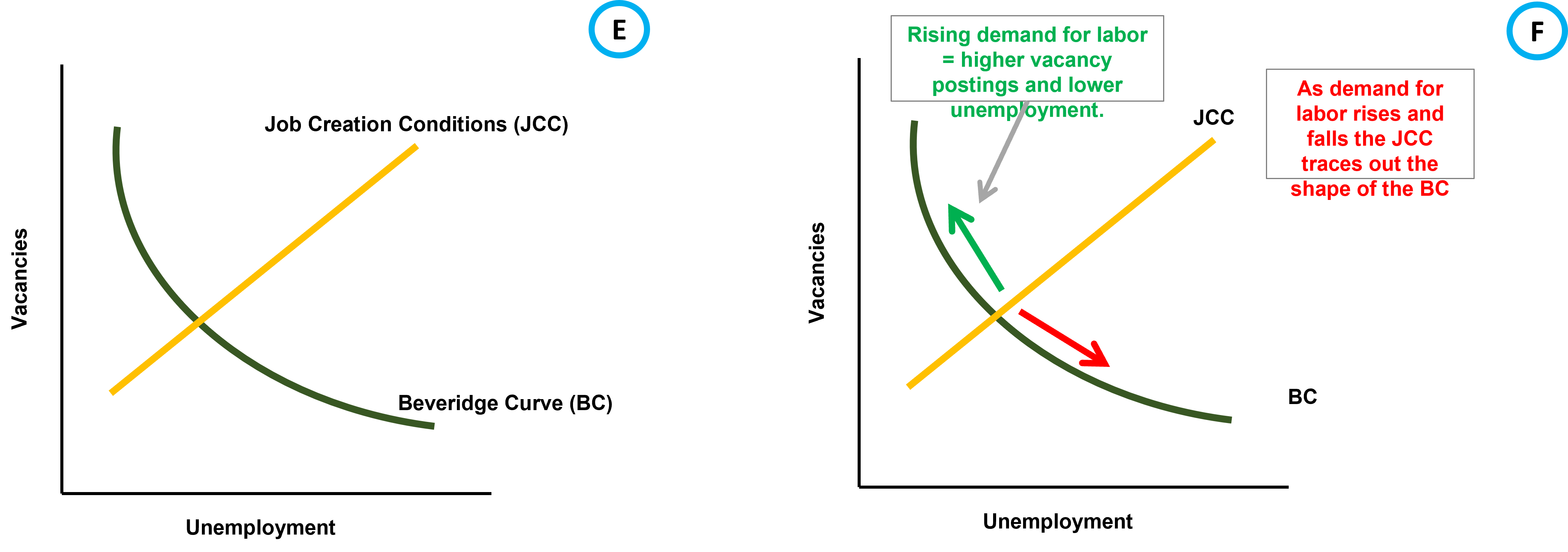
The 1954-1958 cycle was quite simple in its mechanics so to understand the “Beveridge Cycles” that occur after this recession, we must add another component to the diagram - the Job Creation Conditions (“JCC”) curve (Diagram E). The JCC rotates with changes in the demand for labor, which can be interpreted in numerous ways. The two most common methods are: assuming the demand for labor depends on changes in worker productivity, or that demand for labor is driven by revenue per match (“RPM”). The measures used for estimating RPM expectations are all tied to household income, most frequently aggregate employment or aggregate income. When a change in demand for labor is the driving factor, movements of the observed Beveridge curve are the result of changes to the slope of the JCC (Diagram F).
Beveridge Cycles
A “Beveridge Cycle” method views revenue per match as a function of aggregate employment/income, with matching efficiency falling when unemployment is high – due to market congestion. Externalities can cause unemployment and vacancies to never converge to a steady state, but rather move in a closed cycle – a Beveridge Cycle. Expectations of high RPM are self-fulfilling because it stimulates firms to open vacancies, which results in higher employment and higher RPM in the future. However, congestion in a tight market could make hiring so costly that firms reduce vacancies before a steady state is reached. Unemployment rises and RPM falls, causing the process to unwind.
Congestion externalities account for the cyclicality of the Beveridge curve. Matching is less likely if everybody is on one side of the market. Firms expecting lower unemployment should open vacancies immediately because they expect search costs to rise. At the peak of a boom firms overshoot the steady state because of the potential for high RPM. As unemployment reaches cyclical lows the benefits of putting a new employee on the job becomes outweighed by the cost of recruitment. Firms post fewer vacancies than they normally would. Fewer matches are made than jobs destroyed so unemployment rises, causing RPM expectations to fall further – and on goes the process.
The Beveridge Cycle from 1958 to 1961 exhibited a stable Beveridge curve for total unemployment, but the curve for long-term unemployment traces out a counterclockwise rotation (Charts 6 & 7). The only way to explain the exact shape of the curve – with a flat edge early in the expansion and a downward curve as the economy enters recession – is through the interaction of the rotating JCC and the increasing steepness of the Beveridge curve as the labor market tightens.

A New Regime
Beginning in 1982, developments in the vacancy-unemployment relationship changed significantly from the period before. Since 1982, the observed Beveridge curve has exhibited large counterclockwise cycles that have shown the decline in the natural rate of unemployment from cycle to cycle (Chart 8). During the long expansionary periods since 1982 the empirical Beveridge cycle shows a straight line that loops back to become a curve as the economy decelerates (Chart 9).

Conclusion
Using vacancies to forecast changes in business activity has potential, but factors that twist and shift the Beveridge curve must be included in the analysis. The dynamics of the Beveridge curve from 1954 to 1982 were relatively simple and, as a result, the data traces out a textbook curve. The situation started getting more complex after 1982 and the “classic” curve seen in the past disappeared. However, once we incorporate real time shifter the curve suddenly reappears. During periods of transition, the vacancy-unemployment relationship traces out only one piece of a moving and/or twisting curve.
The topic of Part 2 is changes in the labor market that resulted in a new regime for Beveridge cycles after 1982. Changes to the mix of industries and further specialization of individual functions means that today’s labor market is more fragmented than the labor market of the 1950s. Finding the right employee is more difficult and has higher stakes. These factors, among others, have changed the functioning of the labor market and therefore must be considered when analyzing the Beveridge curve (Chart 10).

References
Ahn, Hie & Crane, Leland. (2020). Dynamic Beveridge Curve Accounting.
Diamond, Peter A. and Sahin, Aysegul, Shifts in the Beveridge Curve (August 1, 2014). FRB of New York Staff Report No. 687.
Engbom, Niklas. 2019."Application Cycles,"2019 Meeting Papers 1170, Society for Economic Dynamics.
Ghayad, Rand & Dickens, William. (2012). What Can We Learn by Disaggregating the Unemployment-Vacancy Relationship?
Lubik, Thomas, The Shifting and Twisting Beveridge Curve: An Aggregate Perspective (October 3, 2013). FRB Richmond Working Paper No. 13-16.
Raines, Richard & Jungho Baek, 2016. "The Recent Evolution of the U.S. Beveridge Curve: Evidence from the ARDL Approach," Review of Economics & Finance, Better Advances Press, Canada, vol. 6, pages 14-24, August.
Sniekers, Florian. (2018). Persistence and volatility of Beveridge cycles. International Economic Review.